A graphical explanation of Bayes theorem

by Norman Fenton, Queen Mary University of London

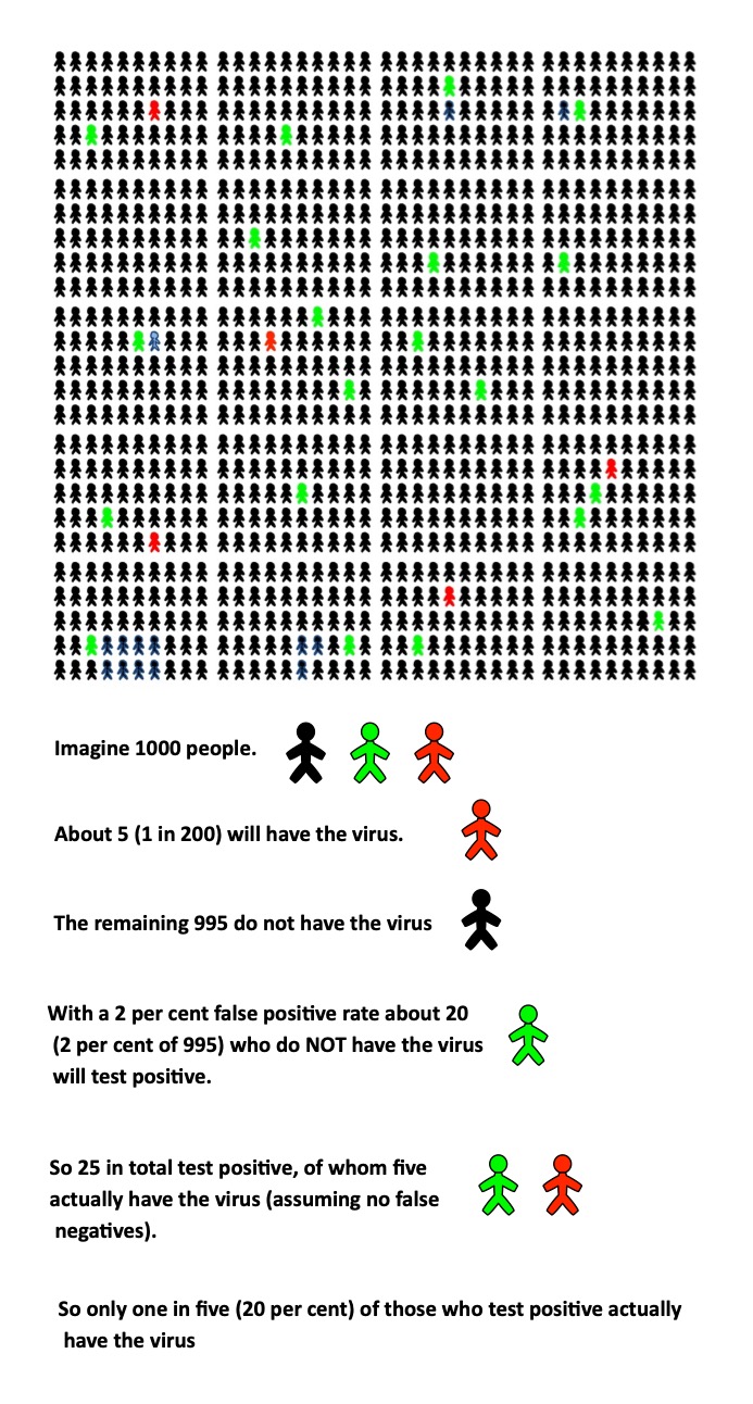
If you take a test how do you work out how likely it is that you have the virus? Bayesian reasoning is one way. Here is a graphical version of what that kind of reasoning is actually about.

If recent data shows that the virus currently affects one in 200 of the population, then it is reasonable to start with the assumption that the probability YOU have the virus is one in 200 (we call this the 'prior probability'). Another way of saying that is that the prior probability is 0.5 per cent.

A better estimate

Suppose the probability a random person has the virus is 1 in 200 or 0.5 per cent. With no other evidence, your best guess that you have the virus is then also 0.5 per cent. You have also however taken a test and it was positive. However, for every 100 people taking the test, 2 will test positive when they actually do NOT have the virus. This means that the false positive rate is 2 per cent.

How? Bayes worked out a general equation for calculating this new, more accurate probability, called the 'posterior' probability (see page 8). It is based, here, on the probability of having the virus before testing (the original, prior probability) and any new evidence, which here is the test result.

A surprising result

How likely is it that you have the virus? With only this evidence, the probability you have the virus is still only 20 per cent.